In the last post, I introduced the fundamentals of Reinforcement Learning and towards the end I discussed the limitations in using traditional tabular methods for learning value and action functions. This motivated the need for using function approximators.

Why Deep Learning?

Instead of having $Q(S, A)$, we parametrize our action function as $Q = f(S, A, \theta)$ where $f$ is a differentiable function which takes $S$ and $A$ as inputs with weights as $\theta$. The idea is to learn the Q-Values by a training procedure similar to a supervised learning setting. Instead of labeled data we will be using the scalar rewards from the environment as the training signal. Since our core objective is to generalize to unseen states, we want to capture the state $S$ into a set of meaningful features related to the task at hand. One way to do this is manually select features which we think captures the dynamics of the problem. We can represent a state in the form $S = \left[ x_{1}, x_{2},…,x_{D}\right]$ and model the Q-function as linear combination of such features.

Now all we have to do is find optimal weights $\theta_{i}$. A straightforward way to do this would be to use the classic stochastic gradient descent used frequently in function optimization. To construct a loss function we can use the TD-target we used in tabular Q-Learning. The loss function can be defined as a mean-squared error of our current estimate and the TD-target from our recent sample.

Let’s say at time step $i$, we transition from state $s$ to state $s’$ by taking action $a$ and we observe an intermediate reward $r$. The loss function for stochastic gradient descent can be constructed as follows,

where $y_{i} = r + \gamma \max_{a’}Q(s’,a’; \theta)$. Now we can update parameters $\theta$ by gradient descent using the gradient $\nabla_\theta L_i(\theta)$. We do this for many episodes and hope that $Q(S, A; \theta)$ converge to $Q_*(S, A)$.

But there two main problems with this approach,

• First, we are manually selecting features. This means our algorithms are task-dependent. We won’t able to build general agents. It is not feasible for a human to hand-engineer features for each task. This is a serious roadblock to achieving human-level intelligence.
• Second, linear combination of features are simply not interesting enough! They severely restrict the agent from learning useful policies required for tackling complicated environments.

This is exactly where Deep Neural Networks enter the picture. Recent breakthroughs in supervised learning like Krizhevsky et all have made it possible to extract meaningful features from just raw sensory data. The idea is to combine Deep Learning methods with Reinforcement Learning so as to solve complex control problems which have high-dimensional sensory input.

But it is not so easy to directly combine deep learning methods with RL because of the way data is generated in RL. The key problems are,

• Deep Learning methods assume large amounts of labeled training data. The only training signal in RL is the scalar reward which is sparse and delayed. An agent might have to wait for thousands of time-steps before it receives any reward. This makes it difficult to generate a strong supervised training signal required for deep learning.
• Deep Learning methods also assume training data to be independent and coming from a fixed distribution. Sequential data from RL by design is extremely correlated and the distribution from which data is generated changes as the agent adjusts its policy.

Because of these two problems, it is difficult to train neural networks for RL problems leading to unstable and diverging learning curves. But Mnih et all. proposed a novel approach called Deep Q-Network(DQN) which overcame these problems and was able to successfully learn super-human policies for various Atari games from just raw pixel data.

Two key ideas which were employed,

• Experience Replay - To break correlation from sequential transitions, the data is stored in a replay memory, and after regular intervals randomly sampled to generate mini-batch required for training using stochastic gradient descent.

• Separate target network - In order to stabilize training, the target required for supervised learning is generated from a separate target network. After regular intervals the target is updated with the agent’s current model parameters. Specifically, The loss function at iteration $i$ is, $L_i(\theta_i) = ((r + \gamma \max_{a’}Q(s’,a’,\theta_{i-1})) - Q(s,a,\theta_{i}) )^{2}$. Note that the target is from $\theta_{i-1}$ which is kept fixed during the optimization process. This deals with the problem of non-stationary targets which causes the neural network to diverge.

Following figure from David Silver’s Deep RL tutorial illustrates the architecture.

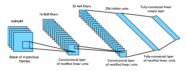
This way DQN provides an end-to-end framework for learning $Q(s,a)$ from pixels $s$. The algorithm was tested on the Atari domain. Inputs from Arcade Learning Emulator are 210x160x3 RGB images which are preprocessed to grayscale 84x84 images. To give the agent a sense of relative motion which we naturally expect in games, the input to the network is a stack of raw pixels from last 4 frames. Output of the network are the Q-Values for 18 possible actions. So one single forward pass for an input $s$ should give $Q(s,a)$ for all actions $a$. The reward is the difference in the game score for the transition. The network architecture and hyperparameters are fixed for all Atari games. Essentially we have one agent learning to play different Atari games to super-human level from just raw pixels without any help from a human.

Policy Gradients and Actor Critic

Though DQN was a major breakthrough in Reinforcement Learning, modern Deep RL methods are leaning towards policy based methods. In DQN, the action function was parametrized as $Q(s,a; \theta)$ and policy $\pi$ was derived as $\pi(s) = \arg\max_a Q(s,a)$. But we can directly parametrize the policy and discover policies which maximize the cumulative reward. The key objective is,

Where $R$ is the cumulative reward you get starting from state $s$. We are directly adjusting our policy to lead to ones which maximize the cumulative reward. The key intuitions in Policy Gradient methods are,

• Collect trajectories $(s_{0}, a_{0}, r_{0}, s_{1}, a_{1}, …, s_{T-1}, a_{T-1}, r_{T-1}, s_{T})$. Push for trajectories which result into good cumulative rewards. Here we define $R = \sum_{i=0}^{T-1} r_{i}$
• Make the good actions which resulted in high rewards to be more probable and bad actions less probable.

In order to optimize, we need a concrete objective function. For DQN, the loss function was defined as mean-squared error of TD-Target and current action function. More importantly we need gradients with respect to our parameters $\theta$ in order to push them towards policies maximizing the cumulative reward. For this we use a score function gradient estimator following derivation from John Schulman’s Deep RL lecture. We are interested in finding gradient of an expression of form $\mathbb{E}_{x \sim p(x | \theta)}[f(x)]$. In RL context $f$ is our reward function, $x$ are our actions sampled from probability distribution $p$, which is the analog for our policy $\pi$.

This gives us an unbiased estimate for our gradient. All we need to is sample $x_i$ from $p(x | \theta)$ and compute our estimate $\hat{g_i} = f(x_i) \nabla_\theta \log p(x_i | \theta)$. If $f(x)$ measures the “goodness” of a sample $x$, pushing $\theta$ along the direction of $\hat{g_i}$ pushes the log probability of the sample in proportion to how good the sample is. From our derivation, this indeed means that we are pushing for samples which maximizes $\mathbb{E}_x[f(x)]$.

This derivation was for one random variable $x$. How to extend this to an entire trajectory we observe in a RL setting?

Consider trajectory $\tau = (s_{0}, a_{0}, r_{0}, s_{1}, a_{1}, …, s_{T-1}, a_{T-1}, r_{T-1}, s_{T})$. We have cumulative reward $R$ defined as $R = \sum_{t=0}^{T-1} r_{t}$. From the derivation we have,

Now we can rewrite $p(\tau | \theta)$ as,

Here $\mu$ is the probability distribution from which start states are sampled. $P$ denotes the transition function (remember MDP!).

Taking $\log$ and $\nabla_\theta$ on both sides,

Plugging this back into our derivation we have,

The interpretation is that good trajectories (ones with high $R$) are used as supervised training signals analogous to the ones used in classification problems. This is a more direct approach to get optimal policies than what we did in DQN.

The above equation is better written in the following way,

This can be interpreted as how we increase the log probability of action $a_{t}$ from state $s_{t}$ in proportion to the total reward we get from state $s_{t}$ onwards; we don’t worry about what happened before $s_t$ for deciding how good action $a_{t}$ is. In practice usually the returns are discounted using a discount factor $\gamma < 1$ to down-weight rewards which are far away in the future.

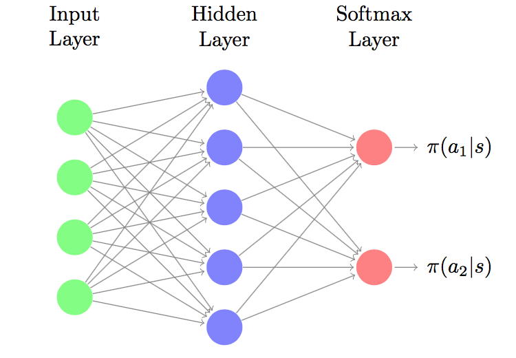
Policy Gradients on CartPole - A pole is attached to a cart which moves on a frictionless track. The objective is to balance the pole on the cart. The pendulum starts in an upright position and the agent has to prevent it from falling over. The agent can apply a force of +1 or -1 to the cart. For each time-step a reward of +1 is provided if the agent manages to keep the pole upright. Episode ends when pole is more than 15 degrees with the vertical or the cart is more than 2.4 units from the center.

Each state is a 4 dimensional input denoting horizontal position, velocity, angular position, and angular velocity. We have two actions applying +1 or -1. The policy $\pi(a | s, \theta)$ is modeled by a 2-layer neural network (with ReLU activation) as shown in figure below,

This is how we we will define a 2-layer network for policy gradients in Python using TensorFlow and Keras,

import tensorflow as tf
import numpy as np
import gym
from keras.layers import Dense, Input
from keras.models import Model

def two_layer_net(inp_dim, out_dim, num_hidden=256, lr=1e-4, decay=0.99):
	states = tf.placeholder(shape=(None, inp_dim), dtype=tf.float32, name='states')
	actions = tf.placeholder(shape=(None, out_dim), dtype=tf.float32, name='actions')
	rewards = tf.placeholder(shape=(None,), dtype=tf.float32, name='rewards')

        # set up the nn layers
	inputs = Input(shape=(inp_dim,))
	fc = Dense(output_dim=num_hidden,activation='relu')(inputs)
	softmax = Dense(output_dim=out_dim, activation='softmax')(inputs)

        # prepare the loss function
	policy_network = Model(input=inputs, output=softmax)
	probs = policy_network(states)
	log_probs = tf.log( tf.clip_by_value(probs, 1e-20, 1.0) )
	log_probs_act = tf.reduce_sum( tf.mul(log_probs, actions), 1 )

	loss = -tf.reduce_sum(log_probs_act*rewards)
	optimizer = tf.train.AdamOptimizer(learning_rate=lr)
	optimize = optimizer.minimize(loss)

	init_op = tf.initialize_all_variables()
	running_reward = tf.placeholder(tf.float32, name='running_reward')
	episode_reward = tf.placeholder(tf.float32, name='episode_reward')
	tf.scalar_summary("Running Reward", running_reward)
	tf.scalar_summary("Episode Reward", episode_reward)
	summary_op = tf.merge_all_summaries()

	model = {}
	model['states'], model['actions'], model['rewards'] = states,actions,rewards
	model['probs'] = probs
	model['optimize'] = optimize
	model['init_op'], model['summary_op'] = init_op,summary_op
	model['running_reward'], model['episode_reward'] = running_reward, episode_reward

	return model

In order to collect trajectories using OpenAI Gym, we do the following,

def run_episode(env, model, sess, actions):
        """
		env - Gym environment object
		model - A dictionary wrapper defining our policy network
		sess - A TensorFlow session object
		actions - action space of the environment
	"""
	x = env.reset()
	xs, acts, rs = [], [], []
	done = False

	state_ph, prob_net = model['states'], model['probs']
	t = 0
        # restricting time-steps to 200
	while not done and t <= 200:
		aprob = sess.run(prob_net, feed_dict={state_ph:[x]})
		act = np.random.choice(len(actions), p=aprob.flatten())

		xs.append(x)
		acts.append(act)  # action (index)

		x, reward, done, info = env.step(actions[act])
		rs.append(reward)
		t += 1


	return [np.vstack(xs), np.array(acts), np.array(rs)]

We need to get discounted returns from each time-step $t$ till the end of the episode. Let us write a function for that,

def discount_rewards(r, gamma):
    """ r: 1D numpy array containing immediate rewards """
	discounted_r = np.zeros_like(r).astype(np.float32)
	running_add = 0
	for t in reversed(xrange(0, r.size)):
		running_add = running_add * gamma + r[t]
		discounted_r[t] = running_add
	return discounted_r

Now that we a have a model and a routine to collect trajectories, we are all set to train our neural network,

def train():
	env = gym.make('CartPole-v0')
	sess = tf.Session()
	K.set_session(sess)
	model = two_layer_net(4, 2, 20, lr=1e-3)
	writer = tf.train.SummaryWriter('cartpole_logs/2layer-Net', graph=sess.graph)

	MAX_UPDATES = 2500
	NUM_BATCH = 4

	avg_reward = 0
	states_ph, action_ph, rewards_ph = model['states'], model['actions'], model['rewards']
	optimize, summary_op = model['optimize'], model['summary_op']
	ep_rwd_ph, avg_rwd_ph = model['episode_reward'], model['running_reward']
	init_op = model['init_op']
	sess.run(init_op)

	T = 0
	while T < MAX_UPDATES:
		batch_s, batch_a, batch_r = None, None, None
		rwds = 0
		for n in range(NUM_BATCH):
			s_n, a_n, r_n = run_episode(env,model,sess,[0,1])
			disc_r = discount_rewards(r_n, 0.99)
			disc_r -= np.mean(disc_r)
			disc_r /= np.std(disc_r)

			r = np.sum(r_n)
			rwds += r

			avg_reward = r if avg_reward is None else .99 * avg_reward + .01 * r

			batch_s = s_n if batch_s is None else np.append(batch_s, s_n, axis=0)
			batch_a = a_n if batch_a is None else np.append(batch_a, a_n)
			batch_r = disc_r if batch_r is None else np.append(batch_r, disc_r)


		_, summary = sess.run([optimize, summary_op], feed_dict={
														states_ph: batch_s,
														action_ph: np.eye(2)[batch_a],
														rewards_ph: batch_r,
														avg_rwd_ph: avg_reward,
														ep_rwd_ph: rwds/float(NUM_BATCH)
			})

		ep_rwd = rwds/float(NUM_BATCH)
		print('Step %d, Episode Reward %.3f, Average Reward %.3f' % (T, ep_rwd, avg_reward))
		writer.add_summary(summary, T)
		T += 1

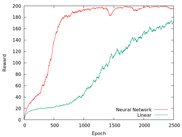
The graph below depicts learning curve averaged over ten trials with a cumulative running reward ($\alpha=0.01$) over epoch (one epoch corresponds to 4 episodes). The maximum number of time-steps per episode was 200. So an optimal policy should get a cumulative reward of 200. One can see the neural network converging to an optimal policy.

Though policy gradient methods provide a direct way to maximize rewards, they are generally noisy with high variance and take too long to converge. The reason for high-variance is we have to wait till the end of the episode and estimate returns over thousands of actions. One way to reduce variance is by adding a baseline. Suppose $f(x) \ge 0$ for all $x$, then for every sample $x_{i}$, the gradient estimate $\hat{g_i}$ pushes the log probability in proportion to $f(x_i)$. But we want good $x_i$ to be pushed up and bad $x_i$ to be pushed down. We can add a baseline $b$ which will ensure that the gradient discourages the probability of all $x$ for which $f(x) < b$. We can incorporate a baseline directly into the policy gradient equation without introducing any bias,

Though by injecting $b$ we don’t introduce any bias, we actually don’t know what $b$ to use. An ideal choice would to be have $b = \mathbb{E}[f(x)]$ because we only want to encourage samples which are above-average. If we don’t know $\mathbb{E}[f(x)]$, we will have to estimate it, and by doing so we will be introducing some bias! This is an example of classic bias-variance trade-off.

Policy Gradients with baseline can be written as,

Actor-Critic methods approximate $b(s_t)$ with $V_\pi(s_t)$, the value function for state $s_t$. They measure how better an action $a$ from a given state $s$ is than what returns the agent would have received if it had followed policy $\pi$, thereby critiquing the actor $\pi$. The policy gradient formula can be refined the following way to incorporate this,

Using $b(s_t) \approx V(s_t)$ and defining the advantage function which critiques the actor as $A_\pi(s,a) = Q_\pi(s,a) - V_\pi(s)$, we have the formula for actor-critic,

Asynchronous Methods

In practice, Actor-Critic methods discussed above are implemented in an asynchronous manner instead of a synchronous approach illustrated in the Python code above. By design policy gradient methods are on-policy. When approximating with neural networks, they still have the same problems as discussed in the beginning of the post : data in a RL setting is non-stationary and extremely correlated. To alleviate these problems, Mnih et al. 2013 proposed an experience replay mechanism. However this restricts the methods to off-policy RL algorithms. Also, experience replay requires more memory and the DQN approach is computationally expensive requiring training over multiple days.

Mnih et all. 2016 proposed an asynchronous variant of the traditional RL algorithms which were backed by deep neural networks. The current state of the art Asynchronous Advantage Actor-Critic (A3C) surpasses DQN while training for half the time on a single multi-core CPU. The key ideas are,

• Replace experience replay with multiple actors training in parallel. This way it is likely that different threads can explore different policies so the overall updates made to the global parameters are less correlated. This can stabilize learning more effectively than a single actor making updates.

• It was empirically observed that reduction in training time is roughly linear with respect to number of parallel actors. Eliminating experience replay means we can now use on-policy methods like SARSA and Actor-Critic.

• Once each actor completes a rollout of their policy, they can perform updates to the global parameters asynchronously. This enables us to use Hogwild! updates as introduced in Recht et al. 2011 where they showed that when most gradient updates only change small parts of a decision variable, then SGD can be parallelized without any locking.

Following figure illustrates the architecture used in implementing Actor-Critic in practice. The following architecture is replicated on each of the actor-threads. Each actor-thread has a local copy of the parameters, which they use to explore the policy and calculate the loss function for the corresponding trajectory. After that, the gradients of this loss function are taken with respect to the global parameters, which are then aggregated over to update them.

The Actor Network and Value Network share most of the parameters. The loss function is combined from the actor and value network. An entropy of the policy $\pi$ is also added to prevent premature convergence to suboptimal policies. This is to give the network an escape route when it is stuck in policies which are bad but are also near-deterministic. For example, let’s say we have an agent with three actions $\langle \text{right, left, stay}\rangle$. If it is stuck in a bad state but the policy prematurely converged to values $\langle0,0.01,0.99\rangle$, it is going to be stuck forever. A nudge to increase its entropy can get the agent out of this.

From Actor-Critic equation described in the last section, we can derive the policy loss as follows,

where $R_t = \sum_{t’=t}^{T-1} \gamma^{t’}r_{t’}$ and the entropy $H(\pi(s;\theta))$ is defined as,

The value loss is defined as,

Combining both, we define the total loss function as,

With this we can set up our neural network model in TensorFlow similar to the way it was done for policy gradients.