I have been studying RL for some time now. It is a very hot field which gained a lot of attention after DeepMind’s agent learned to play ATARI games remarkably well and their AlphaGo bot defeating the Go champion, being the first computer to do so. I have been working through David Silver’s RL lectures, referencing Richard Sutton’s book, and John Schulman’s lectures. I understand things completely only when I write them down and get some Python code running. I want to give a brief intro to RL and dive into writing RL agents with Python. This should be of some help to anyone with no formal background in the area but want to quickly get a mathematical feel about it and start writing agents.

In this post I will talk about

• Building Blocks (MDP, Value Function, Bellman Equation)
• Model Based RL - Dynamic Programming
• Model Free RL - TD Learning
• Q-Learning vs SARSA in Python with Gridworld Example

In the next post I will talk about the Deep Learning variant covering DQN and Policy Gradients to play ATARI games.

So let’s get started!

Building Blocks

Reinforcement Learning (RL) revolves around an agent, which we control, interacting with the environment which is outside of our control. An agent from a given state takes an action on the environment which in turn transitions the agent into a new state and gives a reward.

Our fundamental objective is to build an agent which executes actions so as to get as much reward as possible from the environment. Markov Decision Process helps us in providing a mathematical formulation for this objective. An MDP is a tuple $\langle S, A, P, R \rangle$ where $S$ denotes the state space for the agent, $A$ the action space, $P$ the probability distribution of a transition, and $R$ the corresponding reward distribution. A transition is a sample $(s, a, s’, r)$ observed when an agent from state $s$ takes an action $a$ on the environment and lands in state $s’$ with a reward $r$. Underlying assumption of an MDP is the Markov process. Basically what the Markov assumption means is that the future depends on the present independent of the past. Mathematically,

Value Function in RL is the expected cumulative discounted reward an agent gets from a state following a policy $\pi$. Policy, denoted by $ \pi(a\mid s)$ is the probability that an agent will take action $a$ from state $s$. Policy can be deterministic or stochastic. Deterministic policy is when an agent takes only one action from a given state (probability of taking that action is 1 and everything else is zero).

Mathematically Value Function for a policy $\pi$ is defined as,

Here $G_{t}$ is the total discounted return, defined as $\sum_{k=0}^{\infty} \gamma^{k}R_{t+k+1}$. The discount factor $\gamma$ is an interesting inclusion. The idea is that immediate rewards are more valuable than later rewards. An agent with $\gamma=0$ is considered short-sighted as it aims to maximize only $R_{t+1}$. As $\gamma$ approaches $1$, the agent gives more weight to future rewards. Inclusion of discount factor gives nice mathematical properties required for convergence.

$V_{\pi}(s)$ gives us the average reward an agent receives if it follows policy $\pi$ from state $s$. For a process which has a definite start state and an end state (also called as terminal state), we define an episode as the sequence of transitions from start to end. So if the agent starting from a state $s$ takes part in many such episodes following policy $\pi$ and averages all the total rewards it gets you get $V_{\pi}(s)$. Estimating $V_{\pi}(s)$ accurately is the key challenge in many RL problems and we have different methods depending on how we estimate it.

Action Function is the expected reward an agent gets from a state $s$ having executed action $a$ following a policy $\pi$, it is defined as,

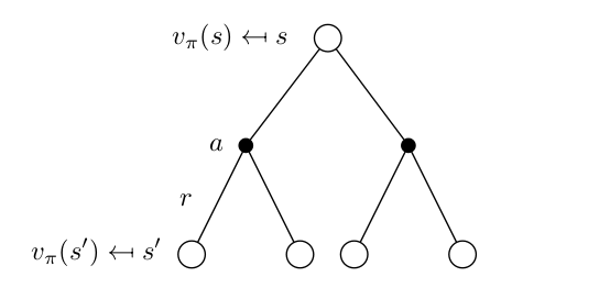
Bellman Equation, one of the most important equations in RL, is a recurrence relation linking the expected reward from current state $s$ and that of next state $s’$. We arrive at a relation by doing a one-step lookahead.

This gives us the Bellman Expectation Equation,

\begin{equation} V_{\pi}(s) = \sum_a \pi(a|s) \sum_{s’} p(s’ | a,s) \left[ r(s,a,s’) + \gamma*V_{\pi}(s’) \right] \end{equation}

From a state $s$, you can chose different actions $a$, each with probability $\pi(a \mid s)$, and once you fix an action $a$, you can go to different states $s’$ with a probability $p(s’ \mid a,s)$ obtaining a reward $r$ in the process. Now what Bellman Equation means is that, average reward you get from $s$ is the expected reward you get in the transition plus the discounted expected reward of the next state. This is indeed intuitve to expect.

This helps us writing value functions in the following way,

where,

Optimal Value Functions - In any RL problem, we are interested in finding the optimal policy. How do we behave in the environment so as to get the maximum rewards? Formally, an optimal policy $ \pi_* $ is a policy for which $V_{\pi_{*}}(s) \ge V_{\pi}(s) ~ \forall ~ s $ for any policy $\pi$. So for an optimal policy $\pi_*$, the value function is,

which can be written as,

An optimal policy has to obey the Bellman Optimality Equation. So to get the optimal action from a state, the one which is going to give us the most reward, we chose the action which maximizes $Q_{*}(s,a)$. It all boils down to finding $Q_{*}(s,a)$.

Here it is essential to understand the difference between prediction problems and control problems. In prediction problems we are interested in finding $V_{\pi}(s)$ and $Q_{\pi}(s,a)$ for all $s$ and $a$ for a given policy $\pi$. In control problems we are interested in finding the optimal policy $\pi_*$ which obeys the opimality equation.

The three important building blocks in a RL problem are

• Model - Which controls the dynamics of the environment affecting the transition probabilities and rewards $p(s’\mid a,s)$ and $r(s’\mid a, s)$
• Value and Action Functions
• Policy - What action an agent must take from each state

Depending on these three categories one can categorize RL algorithms.

Model Based Methods

Now that we have defined the basic building blocks, we can talk about how to solve a Reinforcement Learning problem. By solving, we are primarily interested in two things. One is to know how good a given policy is i.e. what expected reward will the agent get if it follows the policy. This is called as prediction. The second, more important problem is that of control, given an environment, how should the agent behave so as to achieve maximum reward.

In Model Based methods, we assume that we are given the model of how the environment works. Concretely, we are given $p(s’ \mid a, s)$ and $r(s’ \mid a, s)$ for all states and action. Since we know this, we can run a simulation inside our agent’s “head” (also called as planning) and see what action from which state leads to desirable outcomes. Note that the agent is not actually interacting with environment to figure out what works and what doesn’t work. It is just doing a computation in its head to figure that out. This is exactly what we do in an expectimax tree search.

Policy Evaluation is about evaluating a given policy $\pi$. We are interested in finding $V_\pi(s)$ and $Q_\pi(s,a)$. An efficient scalable way to do this is so by an iterative method exploiting the Bellman equation. We know that according to the Bellman Equation,

For $\gamma < 1$ or for eventual termination of all episodes from any state following the policy $\pi$, the existence and uniqueness of $V_\pi$ is guranteed. We exploit the recurrent nature of this equation, thereby giving rise to a Dynamic Programming method.

• Initialize $V(s) ~ \forall ~ s$ arbitrarily. For terminal states $V(\text{terminal state}) = 0$.
• At iteration $k$, for all states perform the update, \(V_{k+1}(s) = \sum_a \pi(a | s) \sum_{s'} p(s' | a,s) \left[ r(s,a,s') + \gamma*V_{k}(s') \right]\)

$V_k(s)$ is the approximate of $V_{\pi}(s)$ and under certain conditions, we can guarantee that $V_{k}$ converges to $V_{\pi}$ as $k \rightarrow \infty$. The algorithm updates the value of $V_k(s)$ by doing a one-step look-ahead into the future to the expected immediate reward it gets plus current estimate of value of the next state. This is an example of full backup boostrapping. Bootstrapping is the process by which we perform our updates based on our current estimate of our return rather than the real return. We call this full backup because we consider all possible actions leading to all possible next states under policy $\pi$ and average over them to perform our update. A process which does not do full backup will only consider a sample of next state, rather than all possible states. Also each iteration updates the value of every state. This is quintessential Dynamic Programming.

So we now have a method to evaluate a given policy. But we are interested mainly in finding the optimal policy. This leads to Policy Improvement.

Policy Improvement is about improving a given policy $\pi$ to a better policy $\pi’$ such that $V_{\pi’}(s) \ge V_{\pi}(s)$ for all states $s$. I will stick to deterministic policies. How do we do this?

Here is when we conisder $Q_{\pi}(s, a)$. Suppose we evaulate $Q_{\pi}(s, a)$ and we figure that it is greater than $V_{\pi}(s)$, this means we are better off with a policy where we select $a$ rather than $\pi(s)$ and then continue following policy $\pi$. We are sure to get more returns under this policy than the policy $\pi$. This is result of policy improvement theorem which states that if $Q(s, \pi’(s)) \ge V_{\pi}(s)$ for all states $s$, then policy $\pi’$ is a better policy than policy $\pi$. That is we can surely say $V_{\pi’}(s) \ge V_{\pi}(s)$ for all states $s$.

Using this result we are going to get a new better policy $\pi’$ by doing the following,

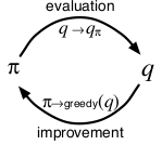
Policy Iteration is about alternating Policy Evaluation and Policy Improvement so that eventually $\pi \rightarrow \pi_*$. In each iteration of Policy Iteration, we do Policy Evaluation to evaluate the current policy $\pi$. This itself may involve several iterations for the values to converge in concurrence with the current policy. Once we complete Policy Evaluation, we perform Policy Improvement, where we do the greedy update as mentioned above. Executing both for several iterations, we are guaranteed that whatever policy we start off with, it eventually converges to the optimal policy $\pi_*$. Of course, the proof for convergence is going to assume certain conditions, which I am not going to get into. But I guess an intuitive understanding is important to get the bigger picture. The following flow image from Richard Sutton’s book explains the process pretty well.

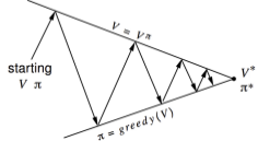
In Policy Iteration, we waited for Policy Evaluation to completely converge to the current policy values and then did our policy improvement step. Since we are interested only in the optimal value function and optimal policies, we don’t need to worry about exact convergence of intermediate policies. We can truncate policy evaluation to few iterations instead of running a complete one. An extreme case of this is Value Iteration. In Value Iteration, after every iteration of our main algorithm, we evaluate our policy and do a policy improvement step. Mathematically,

This is using the Bellman Optimality Equation as an update rule. It can be proved that Value Iteration eventually converges to the optimal values. We can also do this for getting $Q_{*}(s,a)$. This should help us getting the optimal policy for each state. We just max over $a$.

Model Free Methods

The core of Reinforcement Learning is to provide a mathematical framework using which an agent can learn how to perform well in an environment by repeatedly interacting with it by some trial and error mechanism. So far we haven’t done any learning. We just ran a simulation in our head to compute what is good and what is bad. We were able to do that only because a nice oracle gave us how the environment behaves. That’s not how the real world works.

What exactly is the difference between Model Based and Model Free? Let’s take an example. Suppose we want to find the average age of students in a RL course. There are two ways to do it.

• Suppose we know the probability distribution of ages of students in the class. We can simply do the following

  • $ E[\text{age}] = \sum_x p(x)x $

  • Here $p(x)$ is the probability that a student in the class is of age $x$.

• Suppose we didn’t know any such probability distribution, the straightfoward way is to take a sample of $N$ students, and get their average age. We know that for sufficiently large $N$, we will get a very good estimate of average age.

  • $E[\text{age}] = \sum_x \frac{x}{N}$

The second case is what we call as model free. In any real world scenario, we are no way going to get the model of how our environment works. We are not going to get $p(s’\mid s,a)$ and $r(s’\mid s,a)$ in some nice lookup table. A smart agent learns the dynamics of the environment by interacting with it.

How do we make our agent learn? Our agent is going to perform an actual action on the environment and get an immediate reward. We want actions leading to good rewards to get reinforced in a positive way and actions leading to bad rewards to get discouraged. In the previous section, we quantified this with Value Functions and Action Functions. We then calculated them for a given policy and developed a mechanism to improve that policy. We were able to compute this only because we knew the model of the environment - $p(s’\mid a,s)$ and $r(s’\mid a,s)$ in a nice lookup table fashion. In model free methods, we are not going to care about the model. We are still going to work with the Bellman Equation framework BUT we are not going to use $p(s’\mid a,s)$ explicitly (because we don’t know them!). We implicitly learn about $p(s’ \mid a,s)$ in our learning process and never care about explicitly calculating it.

A key point to note here is that we can still do learning with model based methods. If we don’t know the model, we can learn the model! Once we learn the model we can do planning as described in the previous section. But unfortunately model-based methods have not been able to do as well as model-free methods in complicated domains. A recent paper from Silver et al. 2016 Predictron provides an end to end framework for learning and planning

In Monte Carlo methods, we calculate the Value Function and Action Function in a relatively straightfoward empirical fashion by averaging the sample returns. These methods work for episodic problems where there is a clear start state and end state (thereby marking an “episode”).

In Monte Carlo Policy Evaluation,

• For a policy $\pi$, start from state $s$ and follow the policy till you reach the end of the episode. Say you generate a sequence $(S_1, A_1, R_2, S_2, A_2,…,S_{T-1},A_{T-1},R_{T}, S_{T})$.
• For each state $s$ occurring in the episode calculate the return $G_{t} = \sum_{k=0}^{T-1} \gamma^{k}R_{t+k+1}$ obtained from the state till the end and average it. This gives an estimate for $V(s)$.

Repeat the above two steps for as many episodes as possible. It is mathematically provable that the estimate we get for $V(s)$ eventually converges to $V_{\pi}(s)$.

We are literally calculating the average reward we can get from each state under a policy. That is essentially what $V_{\pi}$ is. Pretty straightforward eh?

How do we find the optimal policy? This is where things get interesting.

Whenever we don’t know the model, it is always useful to estimate the action value $Q$, rather than the value function $V$. This is mainly because at the end of the day we are interested in what action to take from each state rather than what reward we get from that state. It is more useful to know $Q_{*}(s,a)$ than $V_{*}(s)$. Why? Knowing $V_{*}(s)$ is pretty useless because we wouldn’t know what action an agent must take from state $s$. For that we have to do a one-step lookahead and arrive at the Bellman Optimality Equation.

We can’t do this because we don’t know the model! We got away in DP because we knew the model and we could afford to do this. But not now. On the other hand if we know $Q_{*}(s, a)$, we can just do,

So in all model free problems involving control the focus is on estimating $Q_*(s,a)$.

We have a MC method to estimate $Q_{\pi}(s, a)$ (exactly same procedure used to estimate $V_{\pi}(s)$). Then we do policy improvement to get a better policy $\pi’$ and keep doing this alternatively to converge at $\pi_{*}$. Thus we may be tempted to think we have a mechanism for finding the optimal policy in model free case. Is that so? Not quite.

The main problem in this case is that while following a policy, we are going to perform one set of actions and that is going to lead us to one set of states. Let’s say we follow a deterministic policy $\pi$. From state $s$, we are going to take only one action $\pi(s)$. While we do MC Policy Evaluation, we will only get an estimate for $Q_{\pi}(s, \pi(s))$ and $Q_{\pi}(s, a)$ for all other actions $a \neq \pi(s)$ wouldn’t improve because we haven’t visited them at all. Now when we do the policy improvement step, obviously only $\pi(s)$ will stand out. So we won’t be effectively improving the policy at all! To improve a policy we have to learn action values for all state-action pairs, not just our current policy. We need to correctly estimate $Q_{\pi}(s, a)$ for all actions $a$ from a given state $s$. How do we do this?

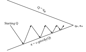
This is the exploration problem. What we do is ensure a continual exploration. We want every state-action pair to be visited an infinite number of times when we execute infinite number of episodes. How we do achieve this? We follow an $\epsilon-$greedy strategy for this. In this strategy we want to ensure $\pi(a \mid s) > 0$ for all $a$. With a probability of $\epsilon$ we select a random action and with a probability of $1-\epsilon$ we select a greedy action. By following this policy, and doing policy evaluation and improvement alternatively, we eventually converge to the optimal policy $\pi_{*}$. Following image from Sutton’s book nicely captures this.

Note that the arrow does not completely touch the top line because we don’t want to completely evaluate $Q_{\pi}$ for each intermediate policy. We are interested only in the optimal policy. An extreme case of this is the Value Iteration in the previous section, where do do evaluation step for only one iteration. For MC methods, after each episode we can have an estimate for $Q_{\pi}(s,a)$ (this wouldn’t have converged to the true value, but we don’t care) and update the policy with policy improvement step. The policy $\pi$ we will be following will be the $\epsilon-$greedy policy.

So we now have a rough idea on how to learn the optimal policy with Monte Carlo Control. But our focus will be on another interesting model free method called TD-Learning.

TD-Learning

TD-Learning combines ideas from both Dynamic Programming and Monte Carlo methods. One main disadvantage in MC methods is that one has to wait till the end of episode to calculate $G_t$. This is a problem in episodes which don’t come to an end. In TD-methods, we update the value of current state based on the estimated value of next state (bootstrapping). In a way, this is exactly what we did in DP. But the difference is that unlike DP, we don’t require the model of the environment. We learn from raw experience by sampling. We don’t do a full width backup like how we do in DP. In DP, we consider all possible actions from a current state and do an update by calculating the average. We are just simulating and planning in the head. But we cannot do this in TD (or even in MC) because once we take an action, on the real world, we are already in the next state. We can’t go back and do another action.

In TD Learning, at its simplest form called TD(0) learning, at every time step $t$ we do

The key idea is that to know how good $V(S_t)$ is, in MC, you had to wait till the end of episode to calculate the true return $G_{t}$. But you already have an estimate of $V(S_{t+1})$ and since $S_{t}$ leads to $S_{t+1}$, it is reasonable to expect that their values are linked in a certain way. If the policy is deterministic and $s$ always leads to $s’$, then value of $s$ is indeed the intermediate reward plus value of $s’$.

The psuedocode for TD(0) to find $V_{\pi}(s)$ can be written as

• Initialize $V(s)$ arbitrarily for all states $s$. Terminal states get $0$ value.
• Run $k$ episodes and for each episode
  • Repeat (till $s$ is terminal)
    • Take action $a$ by sampling from policy $\pi$. Observe next state $s’$ with reward $r$. Do the following update,
    • $ V(s) \leftarrow V(s) + \alpha[r + \gamma V(s’) - V(s)] $
    • $s \leftarrow s’$

We call $r + \gamma V(s’)$ the TD target, value towards which we are updating the current estimate. In MC methods, the target was $G_t$. $\alpha$ here is a learning parameter which controls the degree to which you want to roll in the new information. If $\alpha = 0$, it means you are not interested in the update. If $\alpha = 1$, that means you want to account for the new infromation completely discarding whatever you have learnt before. In practice, a balance is required and affects the degree of convergence of algorithm in use heavily.

Why is this called TD(0)? One thing you may notice is that, we looked only one step ahead when we did the update. But why restrict to only one? Why cant’ we do two steps, like $V(s) \leftarrow V(s) + \alpha[r(s,s’) + \gamma r(s’,s’’) + \gamma^2 V(s’’) - V(s)]$ ? We can. We can even do till the end of the episode! That essentially what we did in Monte Carlo methods. An algorithm called TD($\lambda$) does a tradeoff. How far we lookahead into the future controls how much bias we introduce in our method. When we use $G_{t}$ as the target, it is a true unbiased estimate, because that is what we actually obtained. But when we use $r + \gamma V(s’)$ as the target, we are introducing a bias because $V(s’)$ itself is an estimate, which might be totally random and rubbish initially. MC methods on the other hand tend to have more variance than the TD methods because they wait till the end of the episode to get the update. $TD(\lambda)$ helps in controlling the bias-variance tradeoff.

There is a really nice example from Sutton’s book which illustrates the difference between TD(0) and MC methods when a batch data of experiences is given. In general MC methods converges to estimates which minimize the mean total squared error between the true value and estimated value whereas TD methods converges to a maximum likelihood estimate of the Markov Model which explains the data.

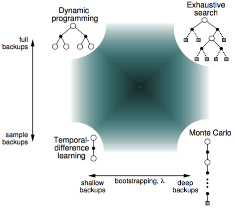
The following diagram from David Silver’s RL lectures presents a unified view of all the models we have discussed so far.

TD-Control: SARSA and Q-Learning

In the previous section we looked at TD-Learning, a model free approach to compute $V_{\pi}(s)$ and $Q_{\pi}(s,a)$. But we are interested in optimal policies, a control problem. So far we have seen that in control problems we alternate between policy evaluation and policy improvement. We calculate $Q_{\pi}(S,A)$ and then do a greedy policy improvement of $\pi$. We also saw that it is not essential to complete policy evaluation at every step because we are only interested in the final optimal policy. The extreme case of this was Value Iteration. We are going to do something very similar for TD-Control as well.

On Policy TD Control: SARSA

In on policy methods, we continually estimate $Q_{\pi}$ for a behavior policy $\pi$ (the policy we actually follow) and at the same time change $\pi$ towards the greediness with respect to $Q_{\pi}$.

The SARSA prediction estimates $Q_{\pi}(s,a)$ with the following update,

The name SARSA (State, Action, Reward, State, Action) is because from a current state-action pair $(S,A)$, we observe a reward $R$, observe next state $S’$, and sample another action $A’$ from policy $\pi$.

For control, we do the following,

• Initialize $Q(S,A) ~ \forall S$. For terminal states $Q(S, .) = 0$.
• Repeat (for each episode)
  • Initialize start state $S$
  • Choose $A$ from $S$ using policy dervied from $Q$ (example, $\epsilon$-greedy)
  • Repeat (for each time step of the episode)
    • Take action $A$. Observe $R, S’$.
    • Choose $A’$ from $S’$ using policy derived from $Q$ (example, $\epsilon$-greedy)
    • $Q(S,A) \leftarrow Q(S,A) + \alpha [R + \gamma Q(S’,A’) - Q(S,A)]$
    • $S \leftarrow S’, A \leftarrow A’$

Does SARSA converge towards $Q_{*}$?

It does if we follow a GLIE (Greedy in the Limit with Infinite Exploration) sequence of policies and we have step-sizes following a Robbins-Monro sequence.

We definie a sequnece of policies $\pi_t$ as GLIE if

• All state-action pairs are visited infinitely many times
  • $\lim_{t \rightarrow \infty} N_t(s,a) = \infty$
• The policy converges on a greedy policy
  • $\lim_{t \rightarrow \infty} \pi_t(a \mid s) = \mathbb{I}(a = \arg\max_{a} Q_{t}(s, a))$

We have Robbins-Monro sequence of step-sizes $\alpha_t$ if

• $\sum_{t=1}^{\infty} \alpha_t = \infty$
• $\sum_{t=1}^{\infty} \alpha_t^2 < \infty$

Qualitatively it means that we want our step-sizes to be sufficiently large so that we can move our action values as much as we want, but changes to the value keeps getting smaller and smaller.

Enough theory, let’s get some code running!

I am going to take Berkeley’s AI Projects to demonstrate a gridworld example with SARSA. They have prvoided a nice gridworld environment for which we can write our own agents. You can find my entire integrated implementation on my github.

We can implement it in the following way,

class SarsaLearningAgent:
	def __init__(self, epsilon, alpha, gamma):
		"You can initialize Q-values here..."
		self.Q = util.Counter()
		self.epsilon = epsilon
		self.alpha = alpha
		self.gamma = gamma
		self.sampleAction = None # for sampling next action in SARSA

	def epsilon_greedy(self, state):
		"""Returns a random action with probability epsilon and greedy action
		   with 1-epsilon"""
		if(random.random() < self.epsilon):
			return random.choice(state.getLegalActions())
		else:
			return self.greedyAction(state)

	def getAction(self, state):
		"Get action from current state using epsilon-greedy policy"
		if self.sampleAction:
			return self.sampleAction
		else:
			return self.epsilon_greedy(state)


	def greedyAction(self, state):
		"Pick the action with maximum QValue"
		legalActions = state.getLegalActions()
		if not legalActions : return None

		qa = [(self.Q[state,action], action) for action in legalActions]
		maxQ, maxA = max(qa, key= lambda x: x[0])
		return random.choice([a for Q,a in qa if Q == maxQ])

	def sampleQValue(self, state):
		""" For SARSA, after we know nextState, we sample an action from the
			current policy, and return the corresponding QValue."""
		if not state.getLegalActions(): return 0 # terminal state
		self.sampleAction = self.epsilon_greedy(state)
		return self.Q[state, self.sampleAction]

	def update(self, state, action, nextState, reward):
		""" Sarsa Bootstrap: Update QValue for oldState,action pair to new reward
			+ estimate of QValue for nextState, sample action using current
			policy. This sample action will actually be taken in the next step
			This is an On-Policy control because update happens towards QValue
			of an action sampled from current policy."""
		alpha = self.alpha
		gamma = self.gamma
		target = reward + gamma * self.sampleQValue(nextState)
		currQ = self.Q[state, action]
		self.Q[state,action] = currQ + self.alpha*(target - currQ)

Here the update() function is called by the environment after every time step.

A sample gif of an agent learning the action values through SARSA ($\alpha=0.2, \gamma=0.9, \epsilon=0.3$):

You get a $+1$ reward if you exit the top right square and a $-1$ reward if you exit the one beneath it. You can see the agent learning from experience.

After $100$ episodes this is what it has learnt,

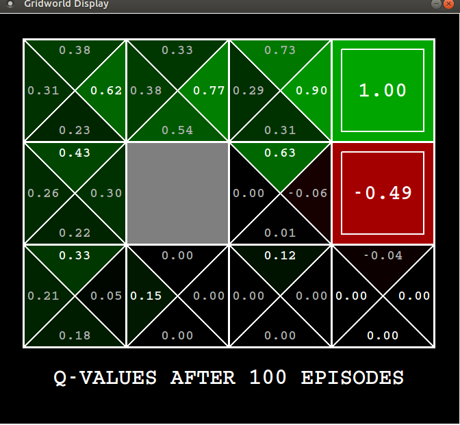
For the top right square, the action value has converged to a value of $+1$. But for the one beneath it, it still remains as $-0.49$, it means the agent has not visited that enough. It doesn’t because we are following an $\epsilon$-greedy policy so $70$% of the time the agent chooses to avoid it because just after visiting it once it has realized that square stinks. Though the action value for other states have not yet converged to the optimal value, you can already see that the agent has discovered the optimal policy.

After $1000$ episodes this is the result,

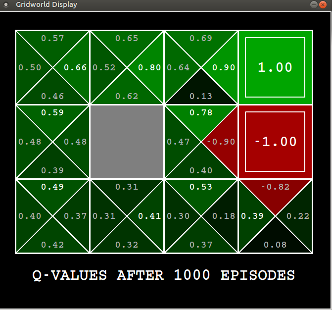
With a discount factor of $0.9$ the maximum reward an agent can get from the top left state is $0.9^3 = 0.73$, our agent has learnt $0.66$, which is pretty close. For some states the action value has converged to $Q_{*}$ and for others it has not exactly converged, but comes close (we are keeping a fixed $\epsilon$ and $\alpha$, so we don’t exactly have the mathematical guarantees).

There can be other environments where if agent arrived at an intermediate policy which causes it to be struck at a certain state, then MC methods will never learn anything, because they wait for the end of the episode to know what return you get. But methods like SARSA which learn from a step-by-step basis figure out that the curernt policy is shit and will learn another policy.

Off Policy TD Control: Q-Learning

In off policy learning we evaluate target policy $\pi(s\mid a)$ while following behavior policy $\mu(a \mid s)$. This is useful when you want your agent to learn by observing other agents. It can also be useful when an agent is learning from its experience generated from old policies. In Q-Learning, the target policy $\pi$ is greedy with respect to $Q(s,a)$, $\pi(S_{t+1}) = \arg\max_a Q(S_{t+1},a)$. So the algorithm is same as SARSA except for the update rule and what next action you take. The update rule is,

In Q-Learning, the update is made towards the optimal Q-Value, but the next action is chosen from $\epsilon$-greedy. In SARSA, the update is made towards Q-Value of an actual action chosen from $\epsilon$-greedy. That is the key difference. The control policy towards which the update is made is the same policy by which the agent is moving but in Q-Learning the update is made towards the greedy policy irrespective of what policy is actually followed by the agent. This is why SARSA is on-policy but Q-Learning is off.

Difference between Q-Learning and SARSA is beautifully illustrated by the Cliff example from Sutton’s book. I will also illustrate the difference with the DiscountGrid environment from the Berkeley AI projects. It is quite similar to the cliff example from Sutton’s book. This is the environment

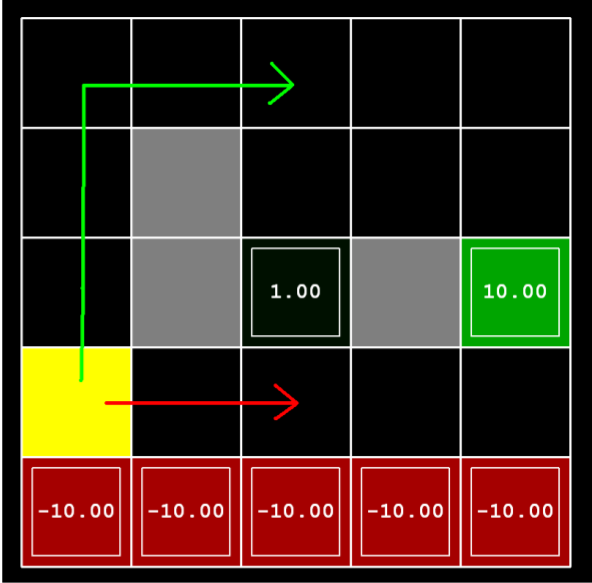
Suppose there are no intermediate rewards and no noise in the environment, the optimal policy is to walk right (red line) towards the $+10$ reward. The roundabout way of reaching $+10$ will be heavily discounted. Let’s see what policies SARSA and Q-Learning agent learn after $10000$ episodes ($\alpha=0.2, \epsilon=0.3, \gamma=0.9$).

Policy learnt by SARSA

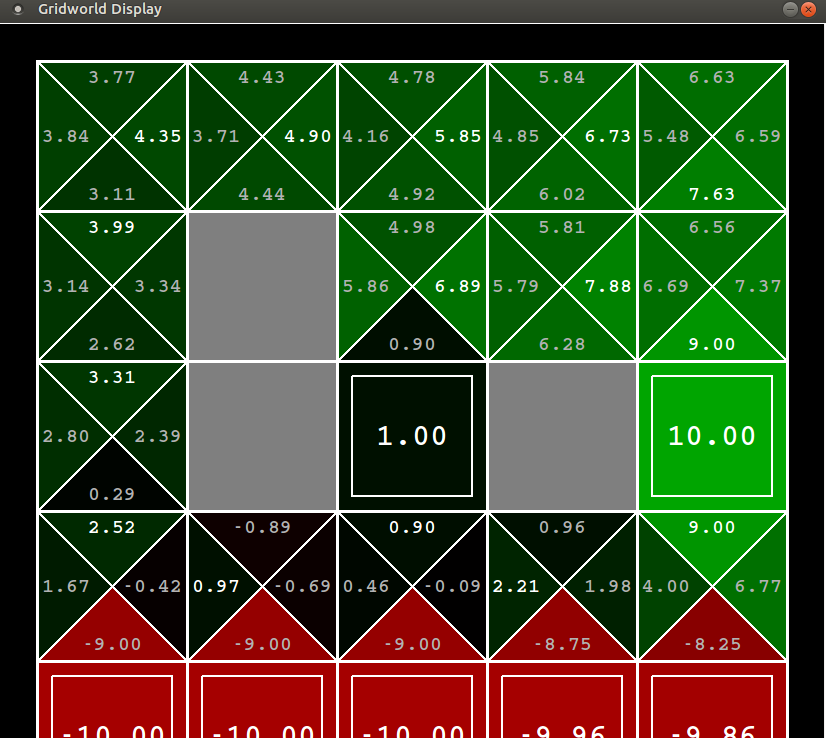
That is after $10000$ episodes if you follow the policy $\pi(s) = \arg\max_a Q(s,a)$ you ssee that SARSA learns the safe roundabout policy. It does this because it follows the $\epsilon$-greedy policy, and it observes that the agent falls into the cliff occassionally which gives it a BIG $-10$ reward. The agent does not like it and realizes that for such a policy with signifcant random component involved, it is better to take the safe roundabout route.

Now look at the policy learnt by Q-Learning

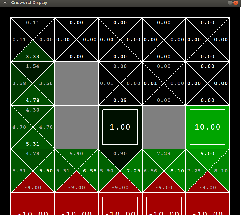
You can see that Q-Learning has learnt the optimal policy. So if you tune $\epsilon$ to zero after the experiment, Q-Learning gives the most reward. Q-Learning is updating its Q-Value towards the greedy policy so is not influenced by the random component invovled in pushing it down the cliff. However since Q-Learning takes the risky route but is actually following the $\epsilon$-greedy policy, it falls into the cliff occassionally thereby giving it a lesser average reward than SARSA.

What’s Next?

This concludes the background chapter for Reinforcement Learning. So far we have been dealing with methods where we directly learn the value function and action function which are stored in tabular format. This approach doesn’t scale to bigger problems for two reasons.

• A lookup table approach will not work effectively for problems having continuous or infinite state spaces. There is finite amount of memory in the RAM. We will quickly hit the ceiling for any interesting RL problem.

• Two different states $S$ and $S’$ might be very similar in structure but from our current methods we will have to learn the value functions for both of them separately. For example, consider a game of PacMan where the agent has just moved one step to the left but everything else in the environment remains in the same. It is reasonable to expect $V(S) \approx V(S’)$, so we shouldn’t have to learn them separately. We want general methods so that we have good estimates for unseen states when we have already visited a similar state in the past.

This leads us to function approximators. Instead of directly learning the value and action function, we parametrize them. This gives our methods the capacity to generalize to unseen state,action pairs.